
Guides
Viewing every kind of data
The Editor's viewer, option by option, for each kind of file a BIDS dataset holds: images, PET, diffusion gradients, spectra, EEG and MEG, physiological and eye-tracking recordings, documents. Every picture is BIDS Manager on the course's converted sample.
Images
Every NIfTI image outside mrs/ opens in the image viewer: anatomical images, functional runs, fieldmaps, diffusion runs, PET.
Layouts
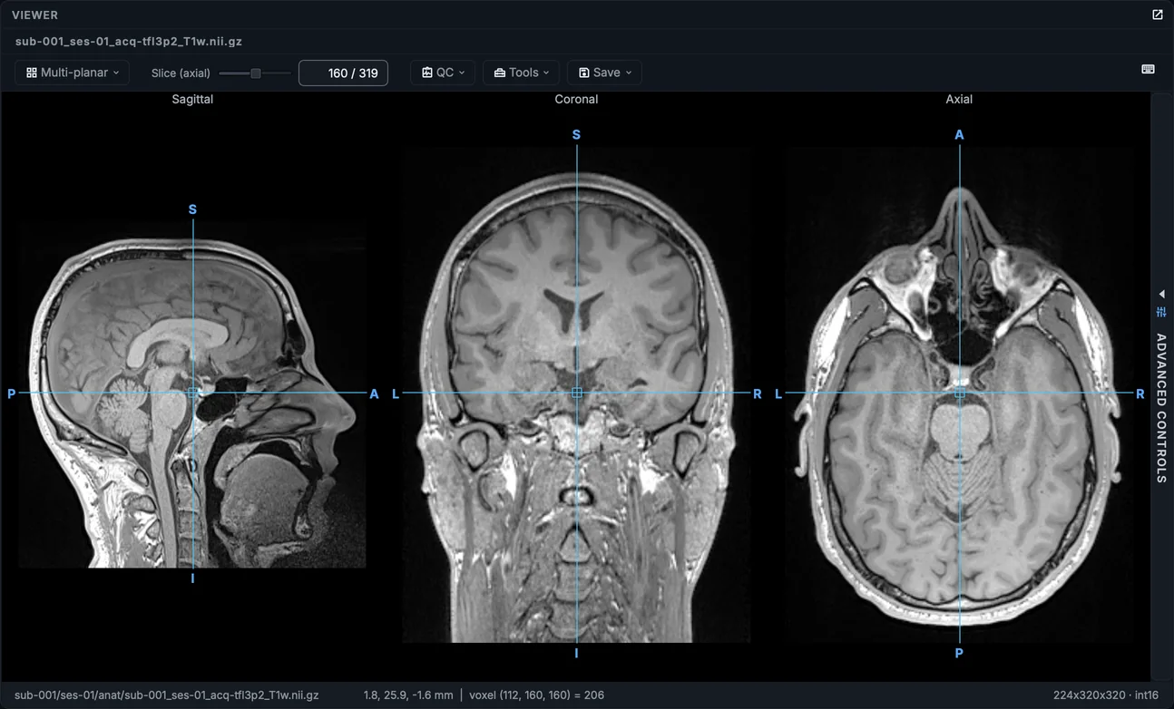
The first button of the viewer's toolbar chooses the layout: one plane; the three planes, sagittal, coronal and axial, sharing one crosshair; a large view with the other planes small beside it; a mosaic of slices; the 3-D rendering alone; or Planes + 3-D, the three planes with the rendering, which is how an anatomical image opens on a computer that can draw 3-D.
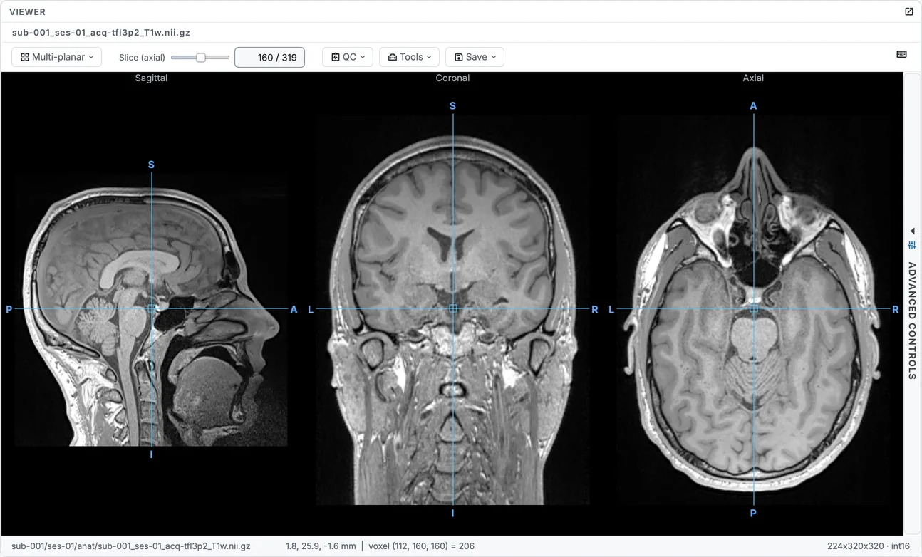
The six layouts, one after the other, on the T1w.
Click in a plane to move the crosshair there, or drag to scrub through the slices; the other planes and the rendering follow. The line under the image gives the position in millimetres, the voxel and its value.
Window, colour map and the other looks of a layer
Advanced controls (⌘I on macOS, Ctrl+I on Windows and Linux), the strip on the right edge of the images, holds everything about how each layer is drawn: the window (the range of values from black to white, with Auto and Full), gamma, the colour map and its inversion, opacity, interpolation, and what to do with values below the window. A change applies to the planes and the rendering together.
Advanced controls beside Planes + 3-D: the colour map changes, in the planes and the rendering at once.
The 3-D view
The rendering is drawn by the graphics card, from the image's own voxels. Drag to turn it, scroll to zoom. Advanced controls chooses its effect: a standard surface, matte, shiny or realistic materials, glass, X-ray, a maximum intensity projection, edges, a shell or a topography; each effect keeps its own parameters, and Reset puts them back.
The 3-D effects, one after the other, with a corner of the head cut away at the crosshair.
Clip planes
Clip planes cut into the volume to show its inside. A plane can cut along an anatomical axis, be tilted to any angle, and move with the crosshair, so the cut follows wherever you click; several planes either crop the volume or cut away only where they all meet, which is how a corner comes out. Corner cut at the crosshair (⇧O on macOS, Shift+O on Windows and Linux) cuts away the corner facing you at the crosshair, the three slices the planes show.
An axial cut through the crosshair moving down, a sagittal cut, then the corner cut at the crosshair.
Overlays and atlases
Tools > Add an overlay... lays another image over the one open: a mask, a statistical map, an atlas, another contrast, a derivative of your own. The overlay is placed by world position, so an image on a different grid lands where it belongs, and it opens with a look that suits what it is: a segmentation or atlas gets one colour per region (named from its _dseg.tsv when it has one), a mask one colour, a probability map a heat map, a map with positive and negative values warm and cool with the small values hidden. Each overlay is a layer in Advanced controls, with its own colour map, window and opacity, and is drawn in the 3-D view too.
The brain from skull stripping laid over the T1w as an overlay, its opacity turned up and down.
Tools also draws a fieldmap of this image over it, steps to the next run, echo, session or subject, and shows the header (below).
Mosaics
The Mosaic layout shows a row of slices at once, each with its position in millimetres. Save > Save a mosaic figure... writes one as a picture; Save also writes a screenshot of what the viewer shows.
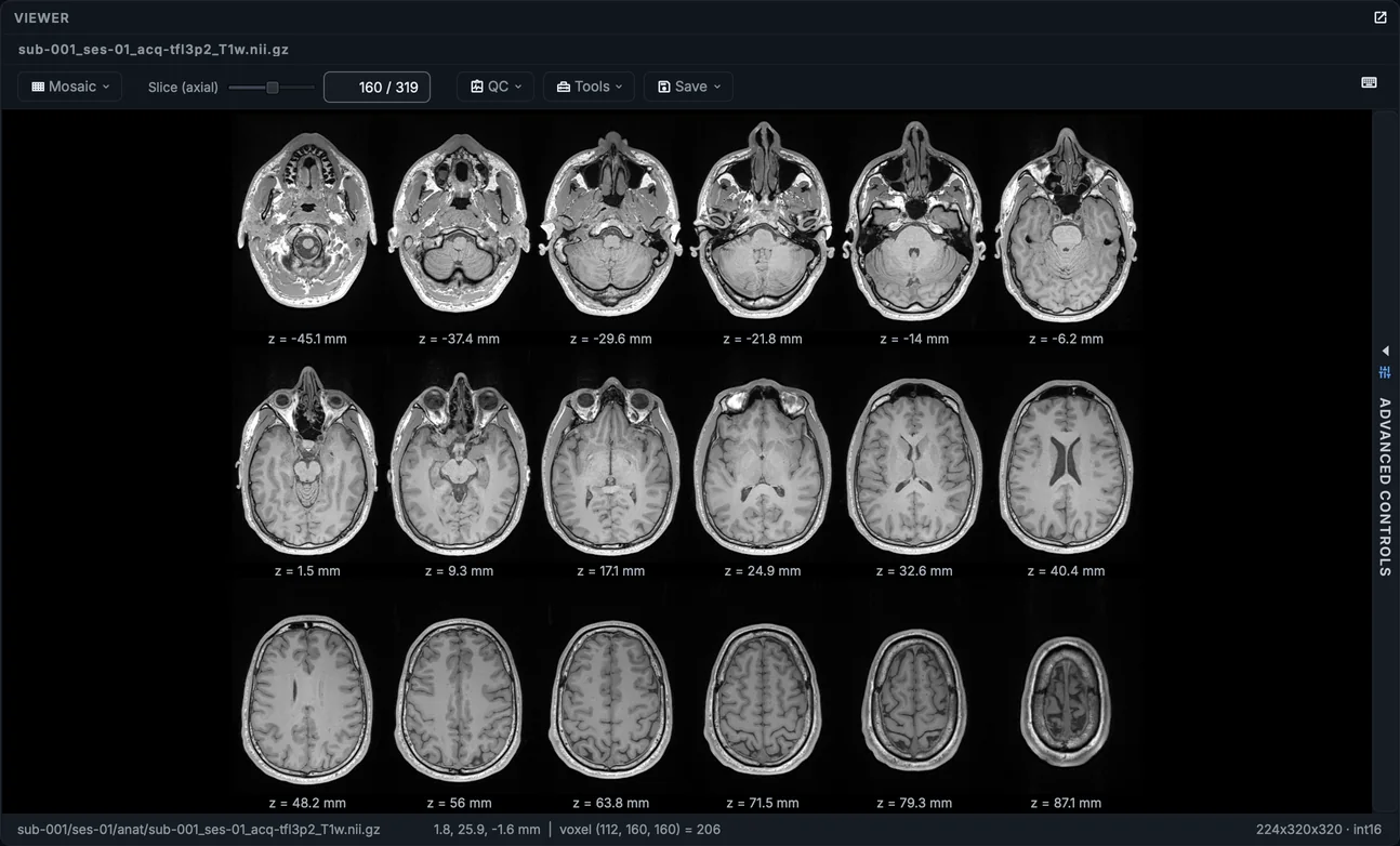
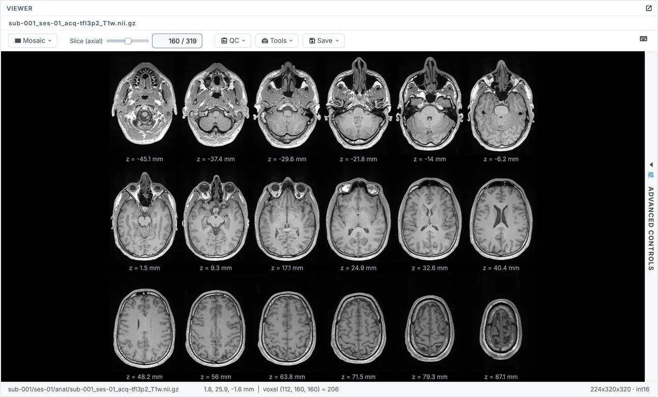
The T1w as a mosaic of axial slices.
The header
Tools > Header shows the NIfTI header beside the sidecar, field against field, so a voxel size or an orientation that disagrees with what the sidecar says is plain to see.
The header inspector of the T1w.
Two images side by side
Tools > Compare images... in the Editor (or right-click (Control-click on a Mac) two images in the tree) opens two images side by side, each with the full viewer; the crosshair, the slice, the plane and the 3-D camera move together, and Same contrast gives both the same window and colour map.
The T1w and the FLAIR, each in Planes + 3-D, turning and moving together.
A time series
A 4-D image (a BOLD run, a dynamic PET) gets Volume and Play in the toolbar, and Time course opens a graph of the signal at the crosshair, in per cent of its mean or in the image's units, against time. For a BOLD run, the graph can carry the run's physiological recordings beneath it, and the quality-check rows: framewise displacement, DVARS, outlier voxels and the carpet plot.
The BOLD run playing, with its time course and the physiological recordings beneath.
The same run with its quality-check rows under the time course.
Quality maps
QC > Check image quality runs the fast quality check on the image open and docks its results beside it; each map the check made (brain mask, tissues, the air measured, the face region) is a checkbox that lays it over the planes and the rendering. Checking image quality explains what is measured.
The quality check of the T1w: grey matter, white matter and the face region laid over the image in turn.
PET
A PET image opens in the same viewer. The hot colour map suits it; a dynamic PET plays frame by frame, and its time course is drawn against the frames' real times in seconds, because PET frames are not evenly spaced.
The PET phantom in Planes + 3-D, in the hot colour map.
Diffusion gradients
A diffusion run's .bval or .bvec opens as its gradient table: the directions on a hemisphere seen along each axis, the b-value of each volume, and the table of volumes; clicking a volume marks it in all three. One checkbox per shell shows or hides it.
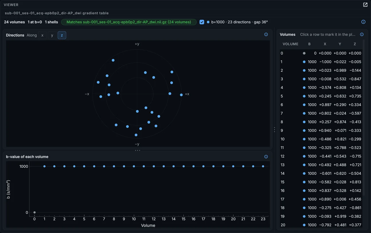
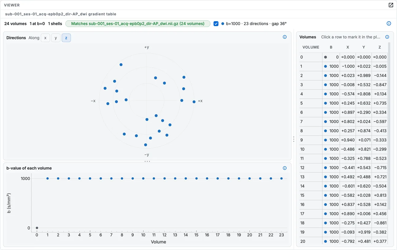
The gradient table of the diffusion run.
MR spectroscopy
A file in mrs/ opens in the spectrum viewer: the spectrum against chemical shift in ppm, drawn from right to left as spectroscopists read it, with the main metabolites marked. Advanced controls sets the component (real, imaginary, magnitude, phase), the repeat shown or the average, the line broadening, and the zero- and first-order phase, which can also be dragged on the spectrum; Auto phase phases it for you. FID shows the signal over time, Water reference draws the water reference with the spectrum, and On anatomy shows the voxel on the anatomical image of the session.
The spectrum phased by hand and set back with Auto phase, line broadening raised, then the FID.
EEG and MEG
An EEG or MEG recording opens on a card with its header (channels, sampling rate, duration); Load signal reads the data. The toolbar sets how many channels are shown, the scaling, the time span and the filter (high-pass, low-pass and notch, applied to what is shown); drag the overview bar at the bottom, or drag the traces, to move through the recording. Advanced controls chooses the channel type or single channels, and Events draws the task's events over the traces.
The EEG unfiltered, then 1 to 40 Hz, then 8 to 13 Hz, with the events drawn and a page forward.
Butterfly draws every channel of a type on one axis, which shows at a glance a moment when they all jump; Normalise scales each channel to its own range.
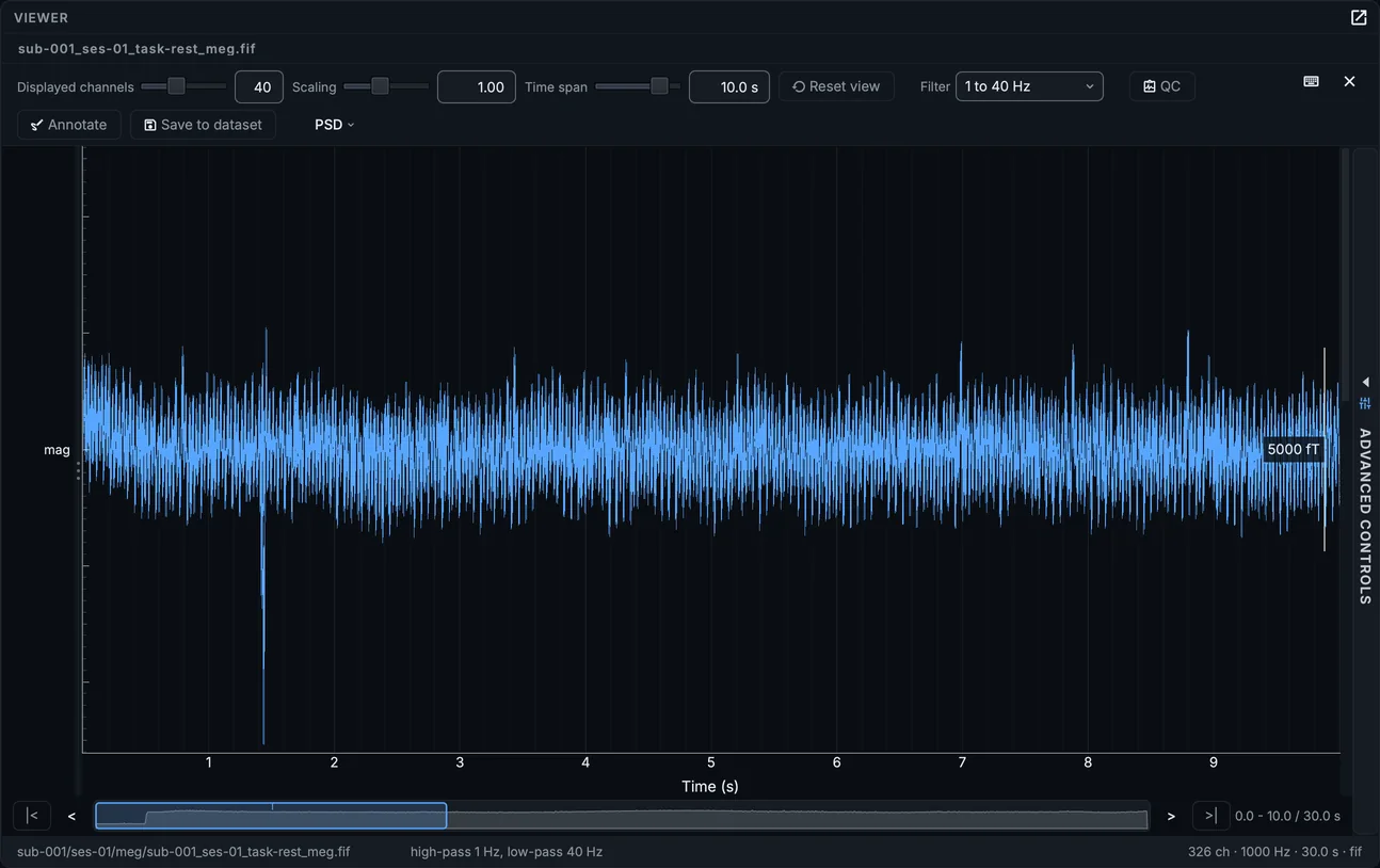
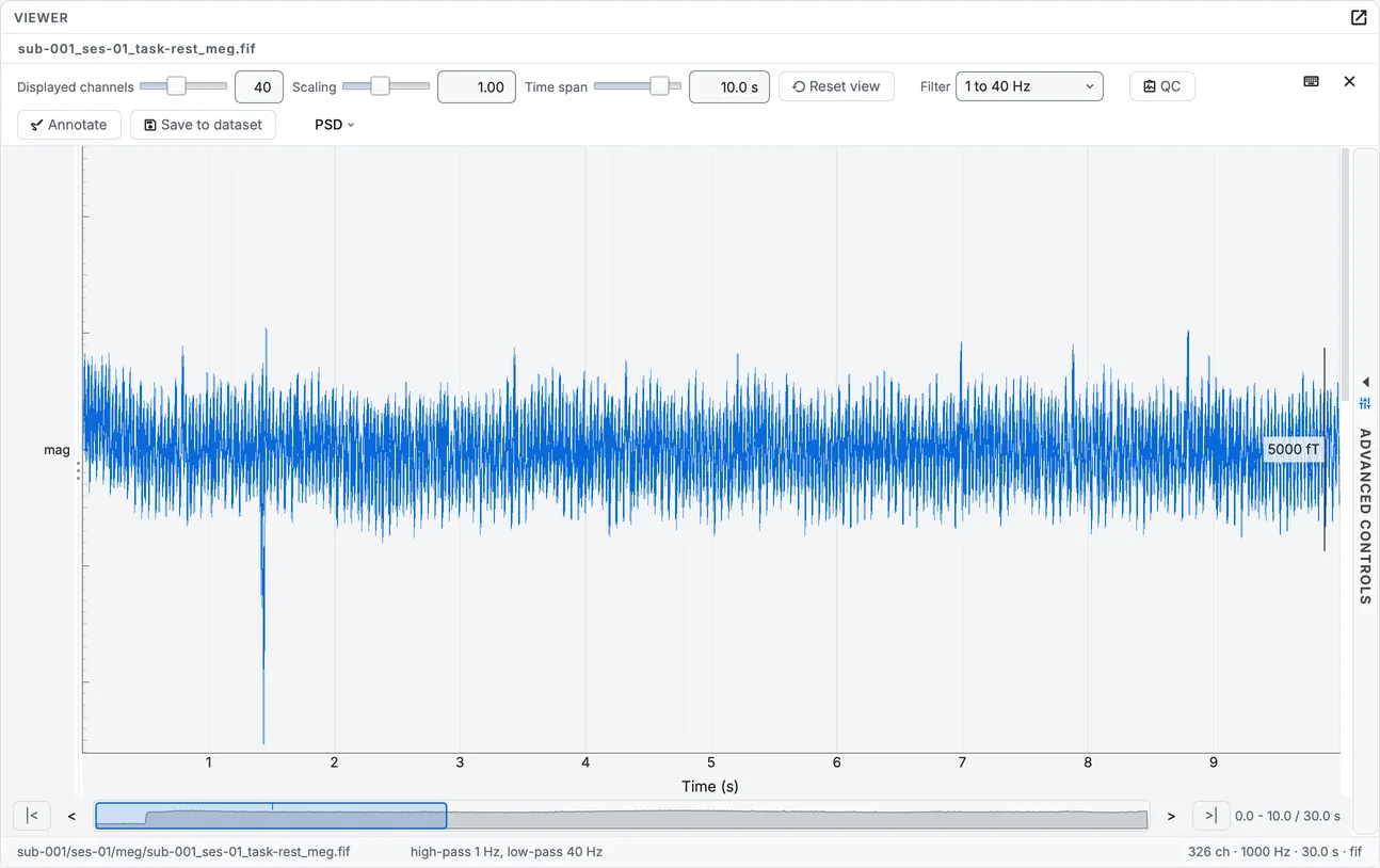
The MEG magnetometers in butterfly mode.
PSD opens the power spectrum: each channel's, or the average per type with its spread, with a crosshair that reads out frequency and power. A line at the power-line frequency (50 or 60 Hz) is the first thing it shows.
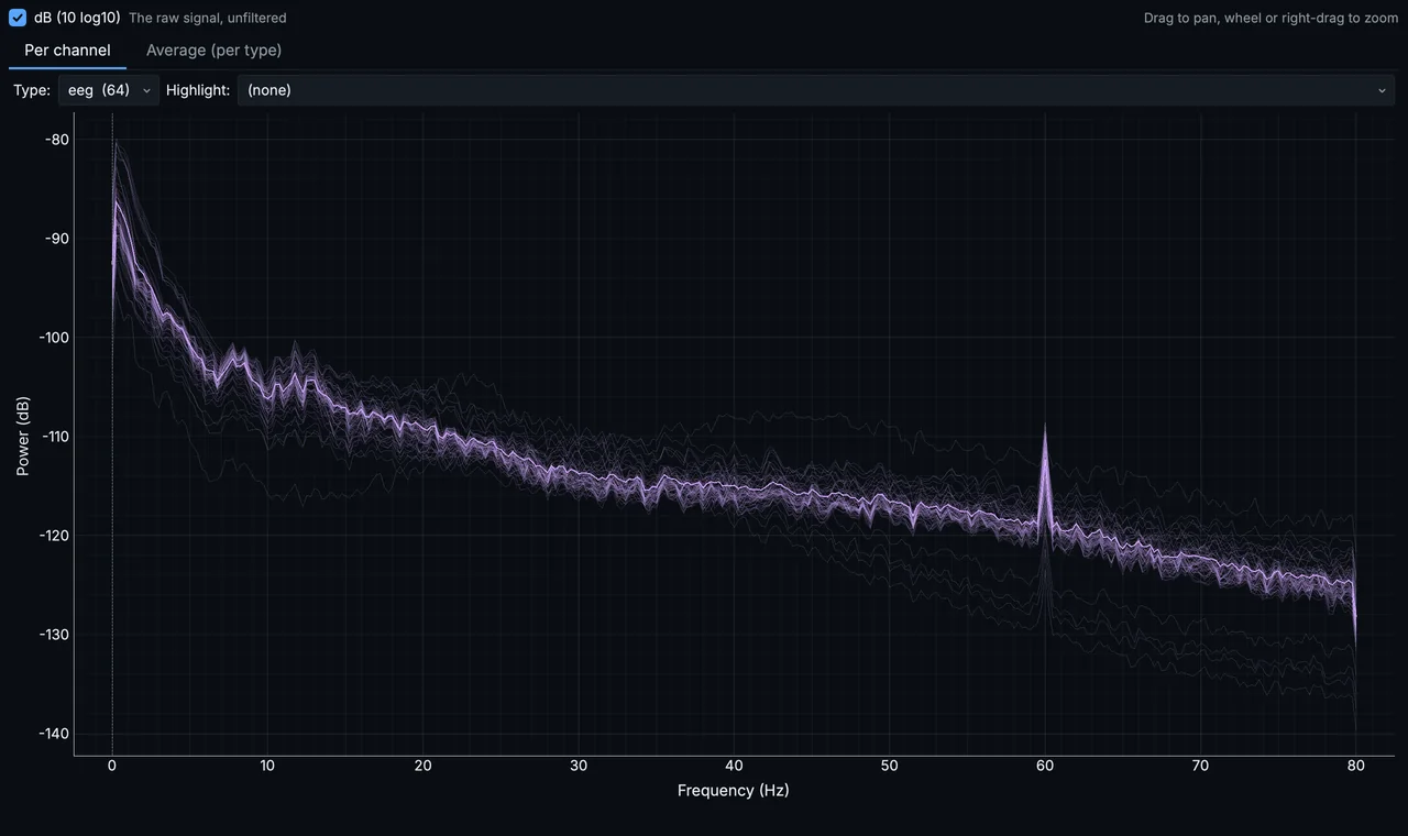
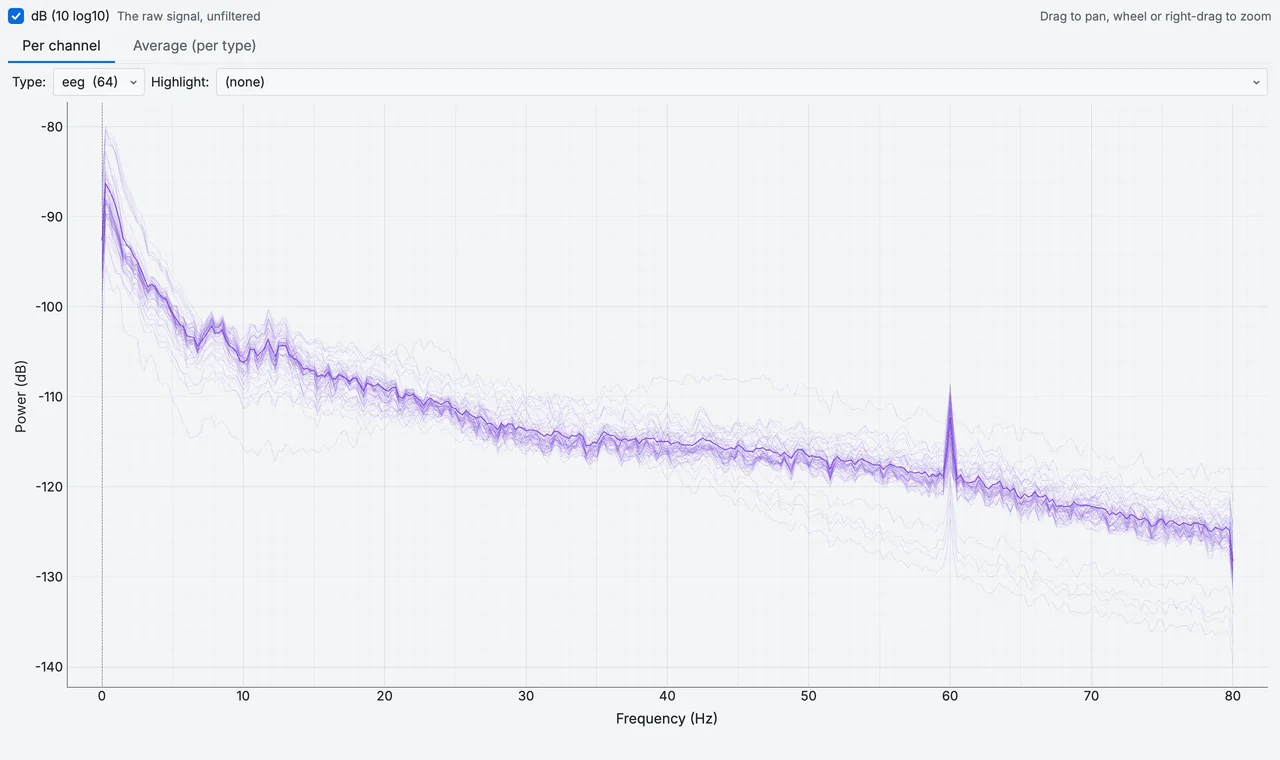
The power spectrum of the motor-imagery EEG: the 60 Hz line of a recording made in the United States.
Annotate turns a drag across the traces into a bad segment, and a click on a channel's name marks it bad; Save to dataset writes them into the recording's events.tsv and channels.tsv, in one operation recorded in the project.
A bad channel and a bad segment marked on the EEG, ready to be saved.
QC checks the recording channel by channel and segment by segment, against the other channels of the same type, and lays its findings beside the traces; each finding can be marked bad from there (Checking image quality).
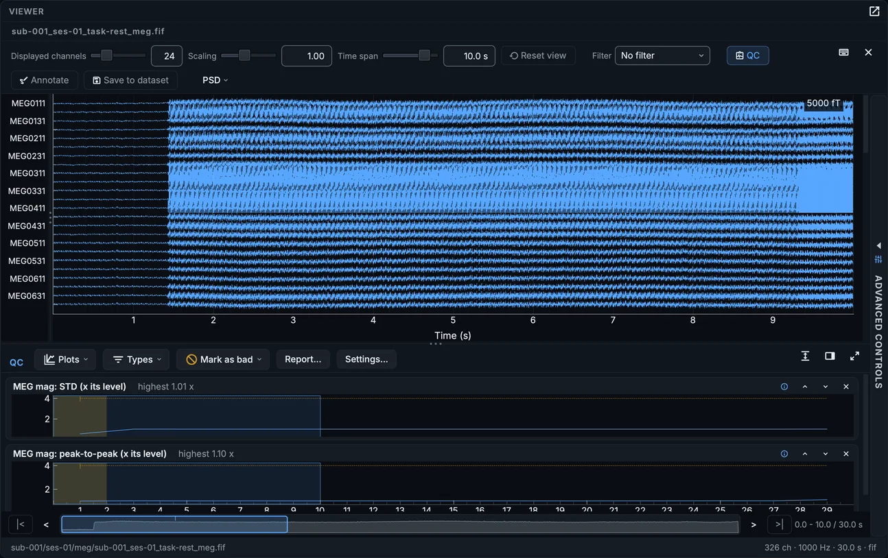
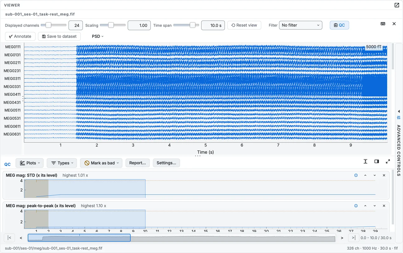
The MEG recording's quality check beside its traces.
Physiological recordings
A _physio.tsv.gz opens as a table; because its sidecar gives a sampling frequency, Visualize draws it in the signal viewer, with the same filters, spectrum and controls as EEG. All of this run draws every physiological recording of the run together, each at its own start time.
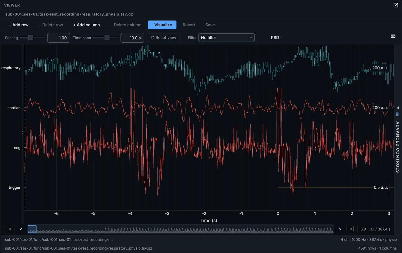
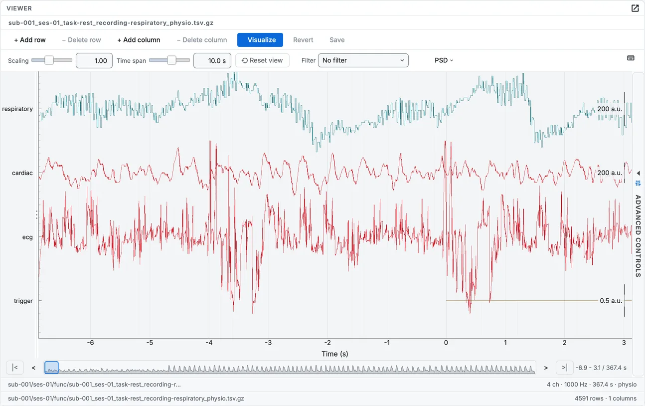
A respiratory recording of the BOLD run, drawn with Visualize.
Eye tracking
Eye-tracking recordings are physiological recordings too, one pair of files per eye: Visualize draws the gaze position and the pupil size, and the gaze traces break where the tracker lost the eye.
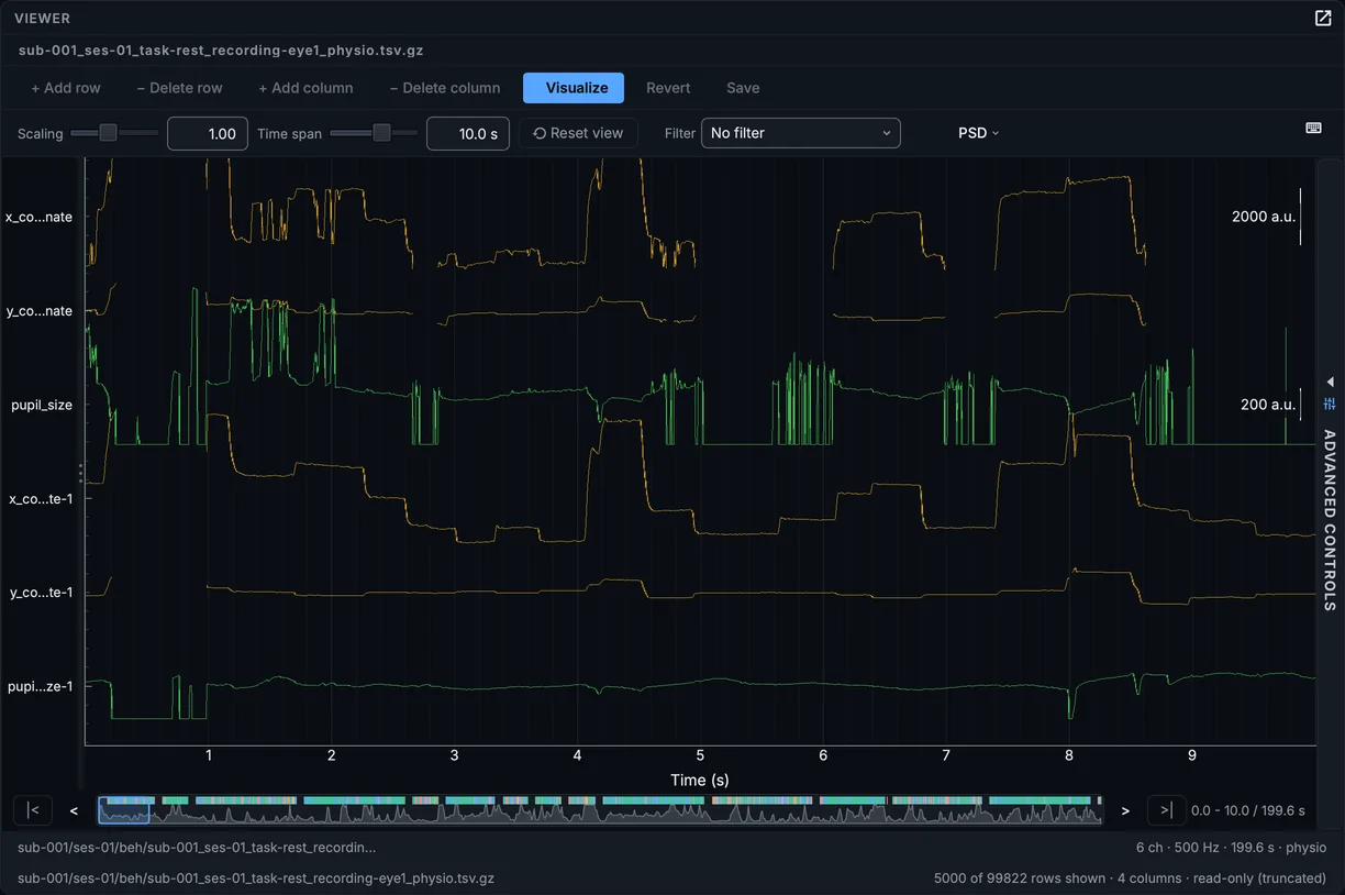
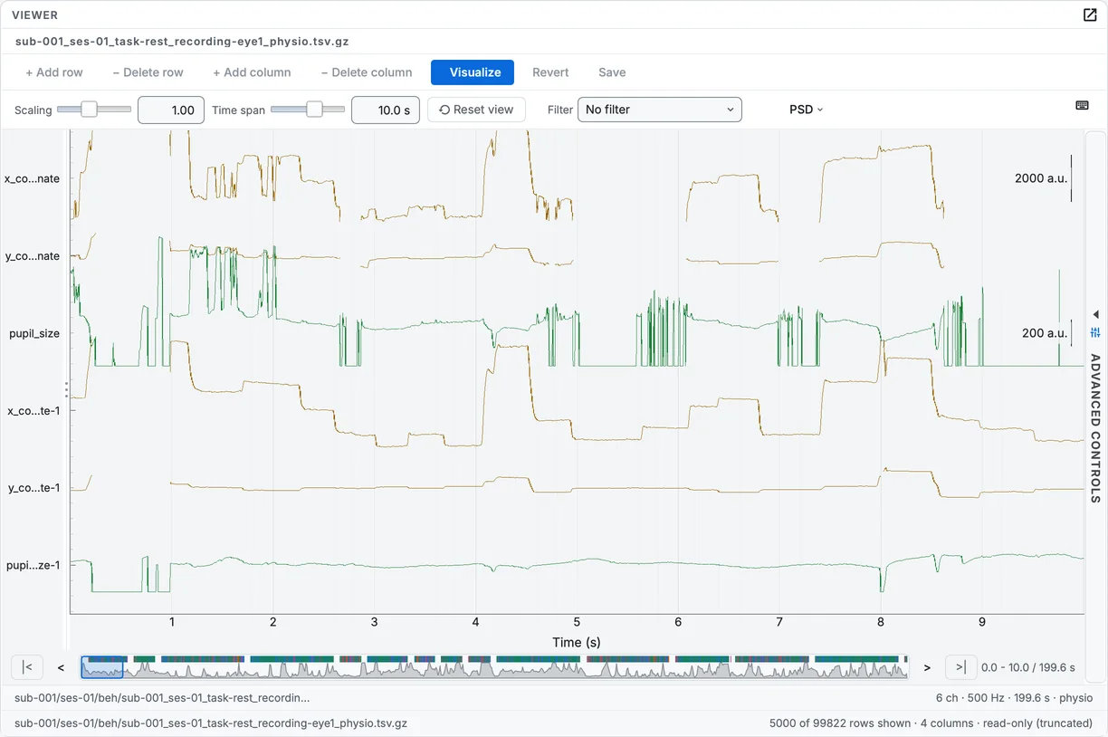
The first eye of the sample's EyeLink recording, drawn.
Documents and tables
README, CHANGES and Markdown files open as text, with Markdown shown rendered; CITATION.cff opens as a form of its fields; JSON sidecars open as forms of their fields, and tables as tables you can edit (Editing metadata). Any other file shows what it is, with a button to open it in your system's own application.
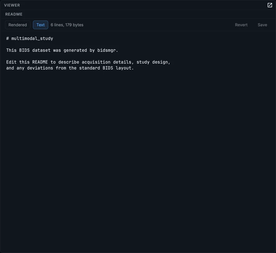
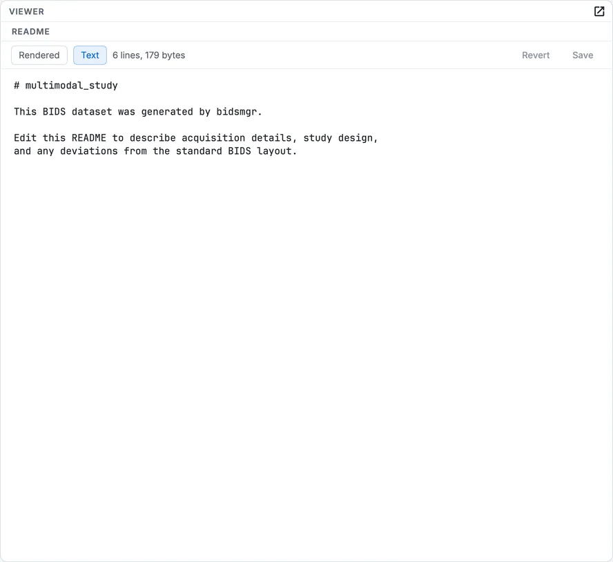
The dataset's README, rendered.