
Learn · Chapter 12 of 15
Viewing data
Look at every kind of file the dataset holds without leaving BIDS Manager. One viewer opens images, signals and spectra; the Editor picks the right one for the file you select.
Images
Step 1. Open the T1w
Select sub-001_ in anat. The Viewer opens it in three planes, sagittal, coronal and axial, sharing one crosshair, and on a computer that can draw 3-D it adds a rendering of the whole volume (Planes + 3-D). If yours does not, choose Planes + 3-D in the layout menu, the first button of the viewer's toolbar.
The T1w in the Planes + 3-D layout. The crosshair moves down through the head, and the corner cut at the crosshair follows it.
Click or drag in any plane to move the crosshair; the other two follow, and so does the 3-D view. Scroll in a plane to step through its slices. Drag in the 3-D view to turn it. The line under the image gives the position in millimetres, the voxel and its value.
Step 2. Change the layout
The first button of the viewer's toolbar is the layout: one plane (axial, coronal or sagittal), Multi-planar, Planes + 3-D, 3-D, Large view and Mosaic, and Layout and mosaic options... to arrange them.
In 3-D, clip planes cut the volume open: the figures here use Corner cut at the crosshair (⇧O on macOS, Shift+O on Windows and Linux), which cuts out the corner facing you at the crosshair, so the cut follows wherever you click. The 3-D view needs a graphics card that supports OpenGL 3.3, which every recent computer has; without it, the 3-D layouts are not offered.
Step 3. Open the advanced controls
Click Advanced controls at the right edge of the viewer, or press ⌘I on macOS, Ctrl+I on Windows and Linux. A column opens with every control, grouped by purpose: the layers and their colour map, window, gamma and opacity; the slice views; the layout; and, in 3-D, its look, clip planes and lighting.
Advanced controls open beside the Planes + 3-D layout: changing the colour map changes the planes and the rendering together.
Tools in the viewer's toolbar adds another image over this one (Add an overlay..., for a mask, a map or an atlas), shows the image's header and sidecar, jumps to the next run, echo, session or subject, and draws a fieldmap that corrects this image over it. Save saves a screenshot or a mosaic figure, saves the look as a preset, saves a scene (what is shown, and how) in the dataset, and shows the command line that reproduces the view with bidsmgr-view.
The viewer remembers how you last looked at each kind of image: a BOLD run opens with its time course, an anatomical image without.
A time series
Select sub-001_ in func. A 4-D image has two more controls in the toolbar: Volume, with Play, and Time course, which draws the signal at the crosshair under the planes.
The BOLD run in the Planes + 3-D layout, playing, with its time course and the run's physiological recordings.
The time course's header sets the Neighbourhood averaged around the crosshair, the Values (raw, % signal change, mean removed) and the Time axis. Physiology draws the run's physiological recordings under it, aligned in time, and QC adds the quality plots of chapter 13.
The diffusion gradients
Select the diffusion run's .bval (or .bvec) in dwi. The Viewer shows the gradient table: the directions on a hemisphere, the b-value of each volume, and the volumes as a table. Click a volume in any of the three to mark it in the others.
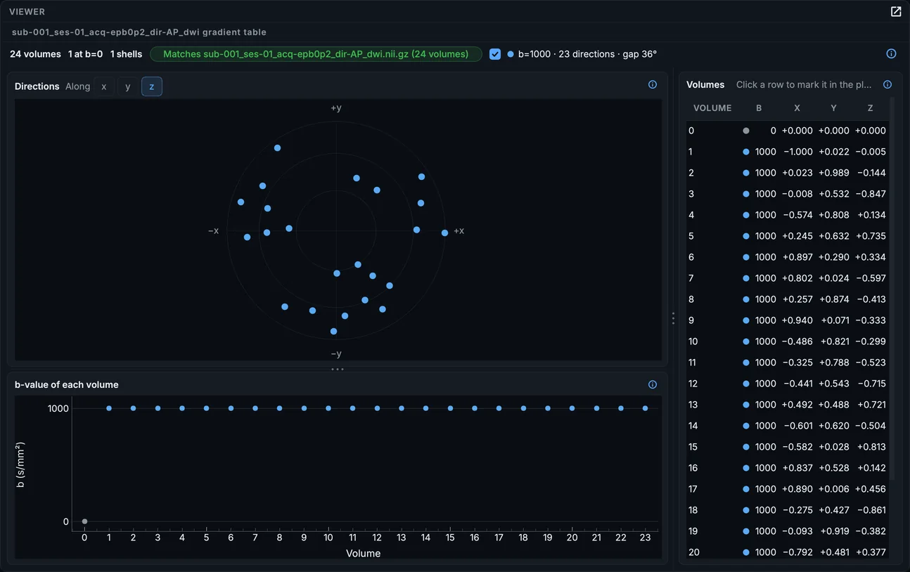
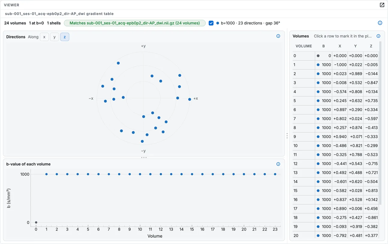
The diffusion run's gradient table.
Signals: EEG and MEG
Select sub-001_ in eeg. The Viewer first shows the recording's header: channels, sampling rate, duration. Click Load signal to read the data.
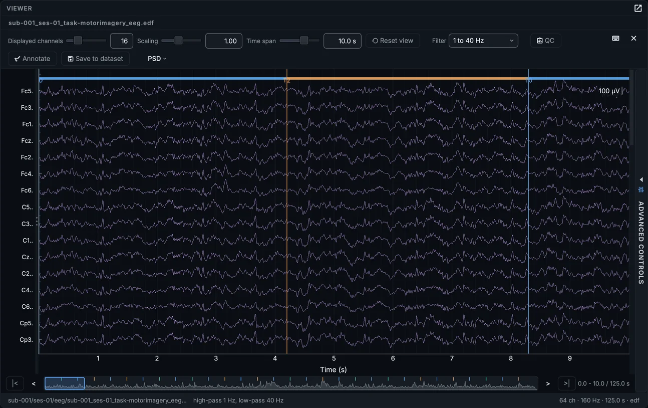
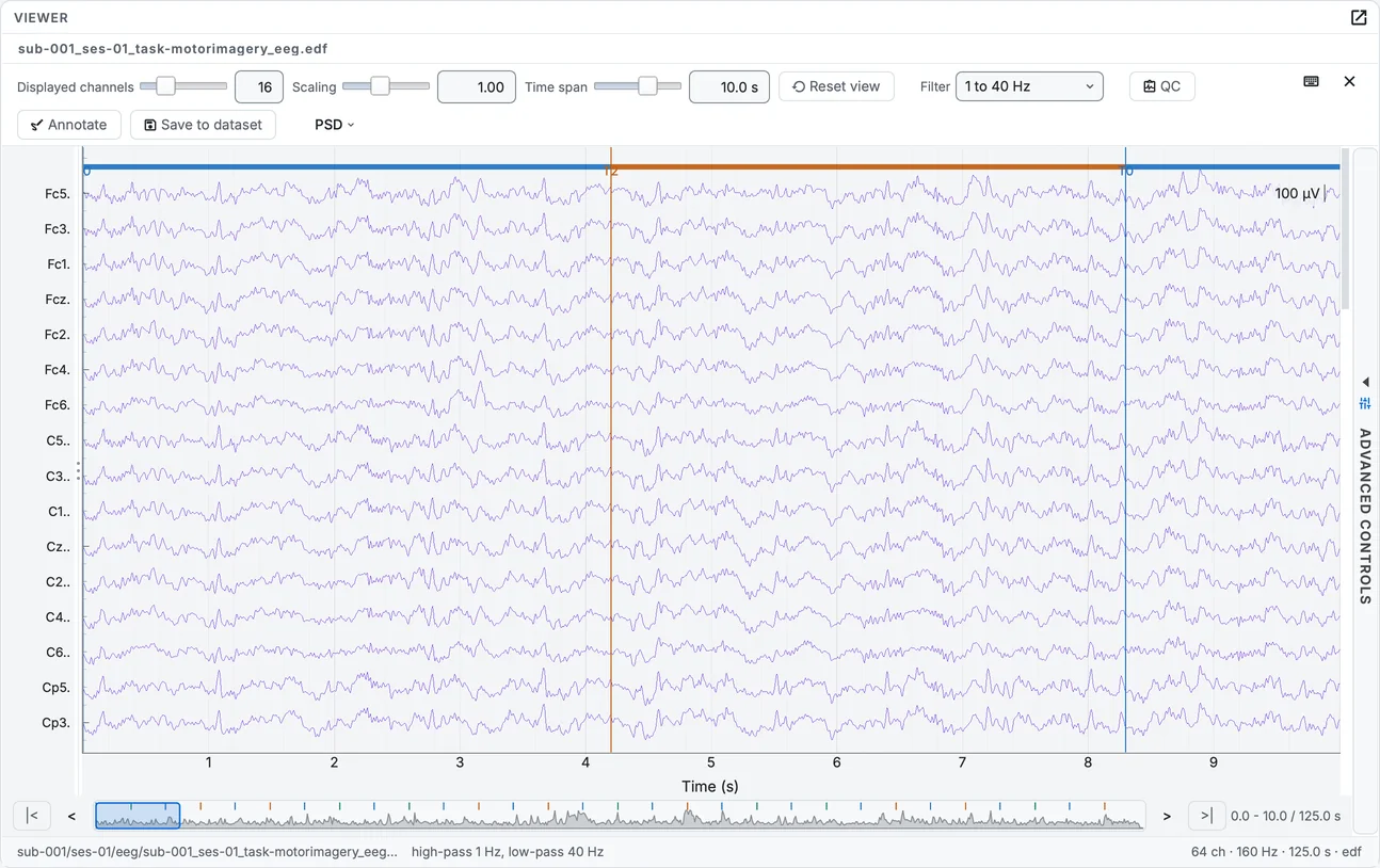
The motor-imagery EEG, filtered from 1 to 40 Hz, with its events.
The toolbar sets the Displayed channels, the Scaling and the Time span, and the Filter. Scroll down the channels, or drag the overview bar at the bottom through the recording. The task's events are drawn as lines over the traces. Annotate marks bad segments and channels, which Save to dataset writes into the recording's events.tsv and channels.tsv; PSD opens the power spectrum.
The MEG recording opens the same way; choose the channel type in the advanced controls, here the magnetometers.
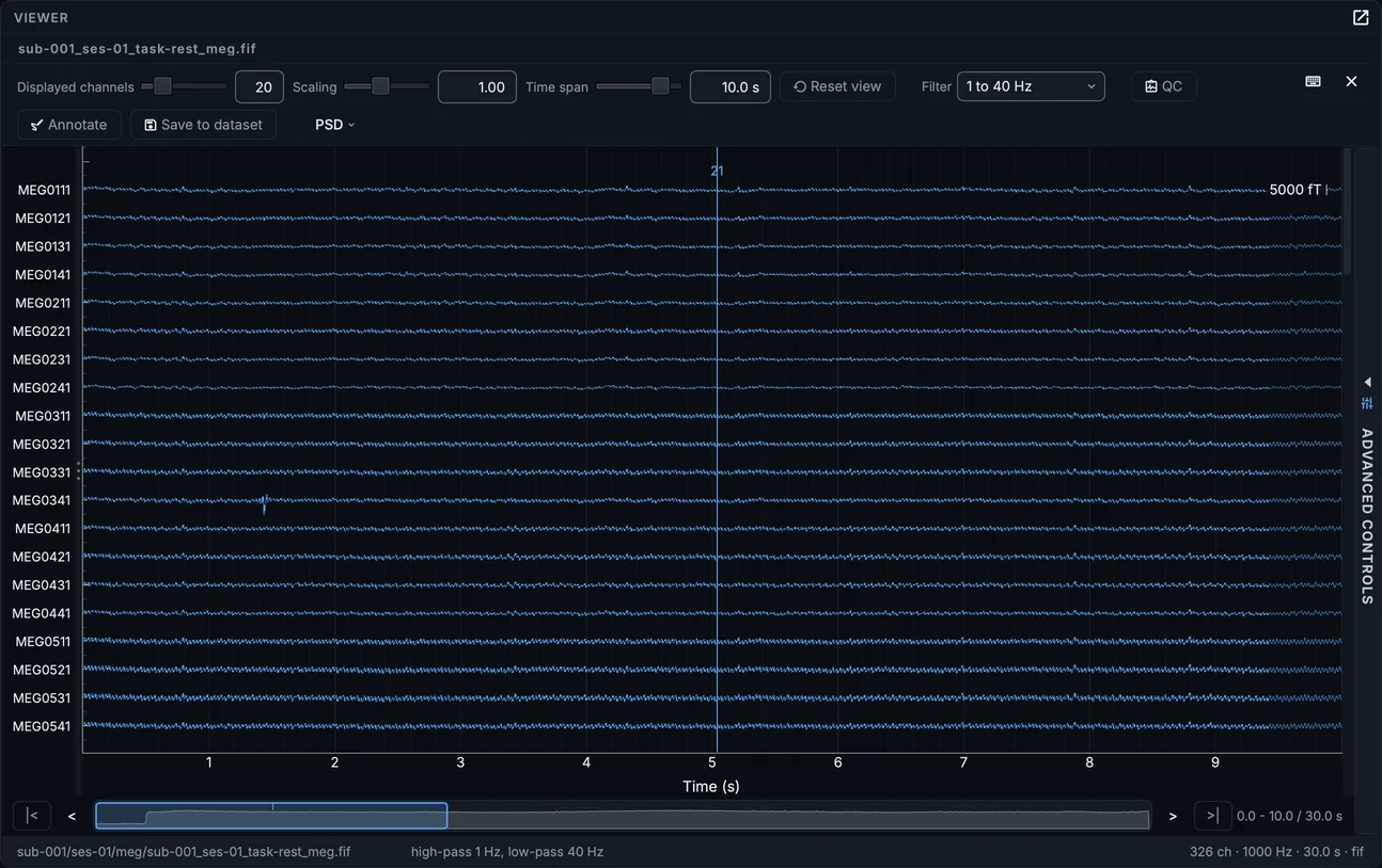
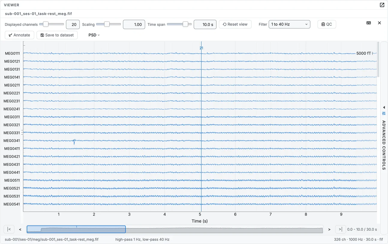
The resting MEG recording, its magnetometers.
Physiological recordings
A _physio.tsv.gz file is a table, so it opens in the table viewer. Because its sidecar gives a sampling frequency, the table viewer has a Visualize button that draws it in the signal viewer: the respiratory, cardiac, ECG and trigger recordings of the BOLD run, each placed at its own start time on one time axis, resampled to the fastest rate among them.
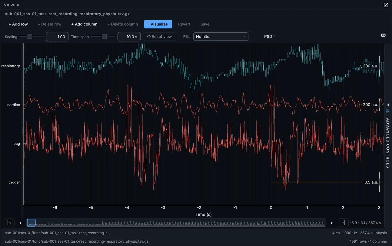
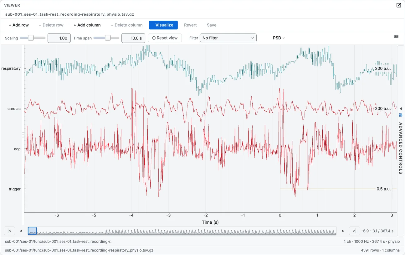
The BOLD run's physiological recordings, with Visualize.
Spectroscopy
Select sub-001_ses-01_svs.nii.gz in mrs. A spectroscopy file is a NIfTI by container only, so it opens as a spectrum: intensity against chemical shift in ppm, drawn from right to left as spectroscopists read it, with the metabolites labelled.
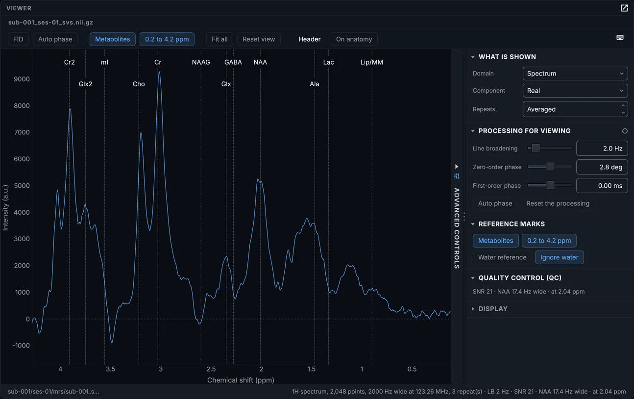
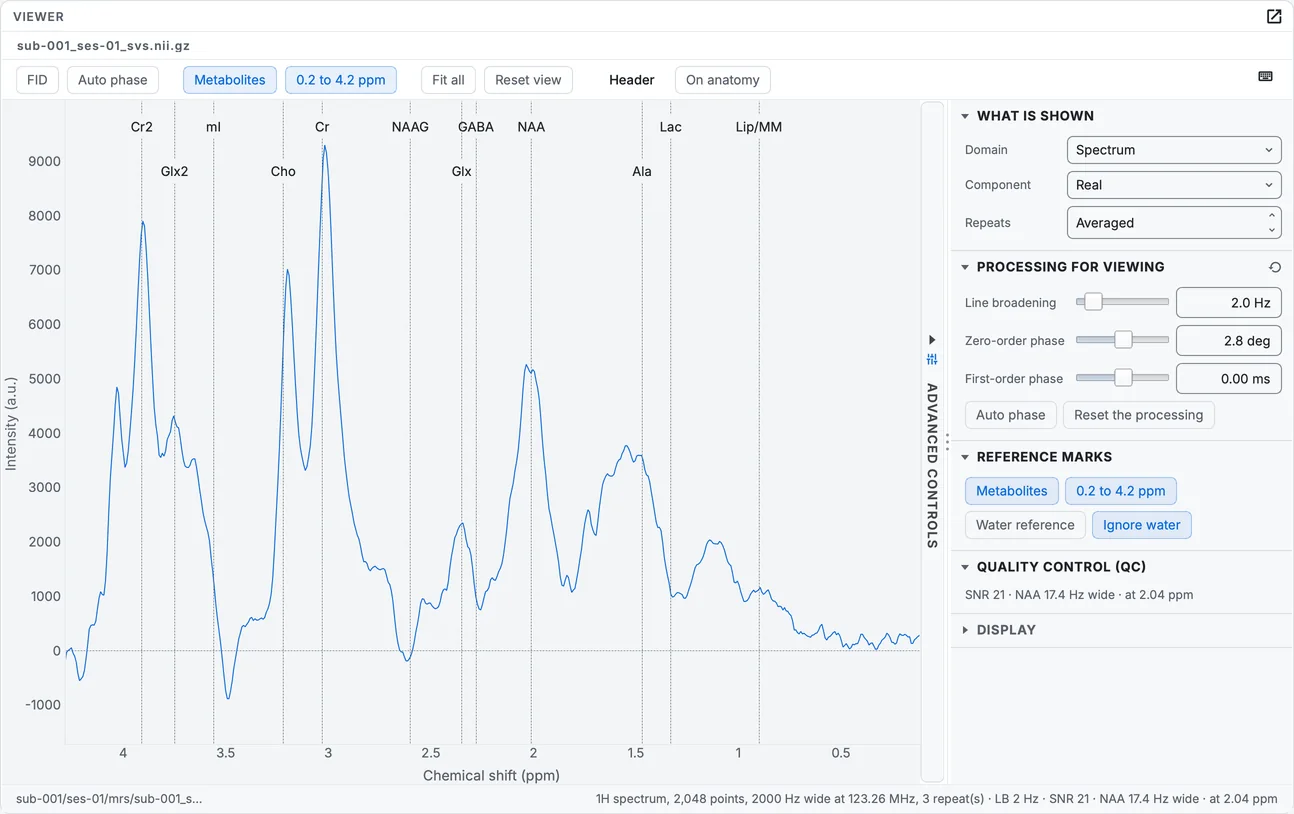
The spectroscopy file as a spectrum.
FID shows the raw signal over time instead; the advanced controls set the line broadening and the phase. On anatomy shows where the voxel was placed on the participant's anatomical image.
PET
A PET image opens in the image viewer like any other; the sample's phantom is one frame. A dynamic PET series gets a time course whose time axis follows the frames' real start times.
The PET phantom in the Planes + 3-D layout, in the hot colour map.
Compare two images
Tools > Compare images... (or right-click (Control-click on a Mac) two images in the tree and Compare these two images...) shows two images side by side with one toolbar: the crosshair, the slice, the plane and the 3-D view move together; tick Same contrast to give both the same window and colour map as well.
Comparing the T1w and the FLAIR, each in the Planes + 3-D layout: they turn and move together.
Keys and gestures
The viewer's shortcuts are listed under the keyboard icon at the right of its toolbar, and in Viewers in the Reference, written for your system. Settings > Viewer shortcuts changes them.
Your progress is kept in this browser only.